gvSIG-Desktop 1.10. User Manual

When you click on the “Geoprocessing wizard” button, the following dialogue appears:

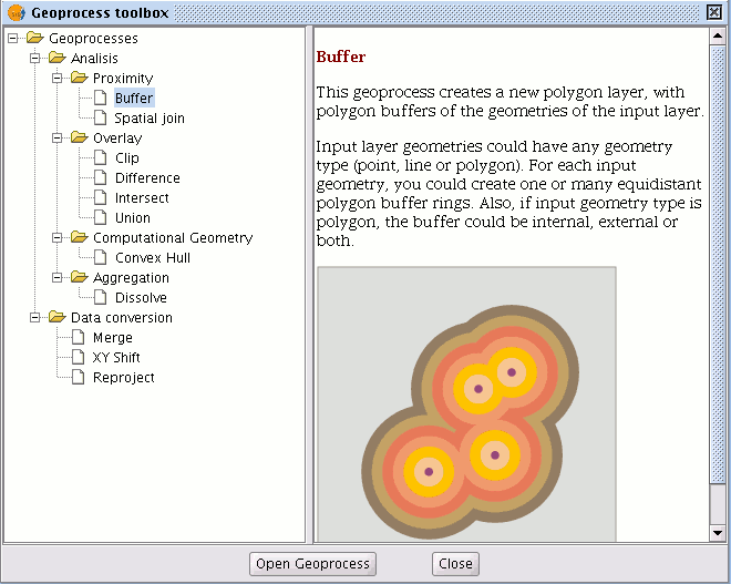
If you select “Buffer” and click on the “Open geoprocess” button, the window associated with this process is shown:

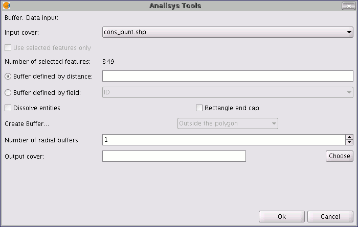
The form is divided into the following parts:

Selecting the elements whose buffer is to be computed. This is a pull-down list in which you can select the vector layer the calculation is to be applied to. If you wish, you can enable the “Use selected features only” check box so that the process only computes the buffer of the elements currently selected in the specified layer.

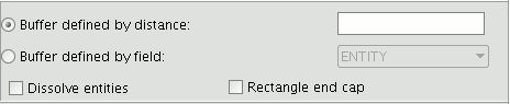
Inputting the features of the buffer to be computed. You can choose to input the buffer defined by distance (in the first text box) or to input a field in the input layer, from which the buffer radius value to be applied will be taken. This second option allows you to apply different buffer radii to different vector elements (whilst the first option applies the same radius to all the elements in the input layer). When the buffer of all the input layer elements has been generated, the “Dissolve features” option allows you to merge the elements whose geometries touch each other in a second iteration.

The “Rectangle end cap" option allows you to generate buffers with perpendicular edges (not rounded). Selecting the number of concentric buffers and their situation regarding the original geometry. The gvSIG “Buffer” geoprocess allows you to generate several equidistant areas of influence of the original geometry (for example, if the buffer distance to be applied is 200m and you choose to generate two concentric radial rings, the buffer distance of the second ring will be between 200-400m. Currently, you can only generate a maximum of three concentric radial buffer rings for efficiency reasons. If the vector layer we are working on is a polygon layer, the “Create Buffer…” option will be enabled, thus allowing the user to generate buffers outside, inside and both inside and outside the original polygon.

Introducing the result layer characteristics. Currently, the result of running a geoprocess can only be saved as an shp file. Thus, gvSIG allows you to select an existing shp file to overwrite it or to specify a new one. As new formats are supported to save the result of the geoprocesses, wizards will be provided to indicate the characteristics of these formats.

When you have input all the necessary information to compute the buffer, and clicked on the “Ok” button, a check routine is carried out to ensure that the information input is correct: whether the radius distance is numerical, whether the attribute from which the buffer radii are taken are numerical, whether a result file has been input, etc. If the check routine is not correct, a dialogue box appears so that the input data can be corrected.

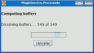
If the input information that you have entered is correct, a window with a progress bar appears, in which the buffer processing rate is shown.

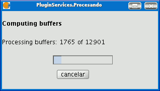
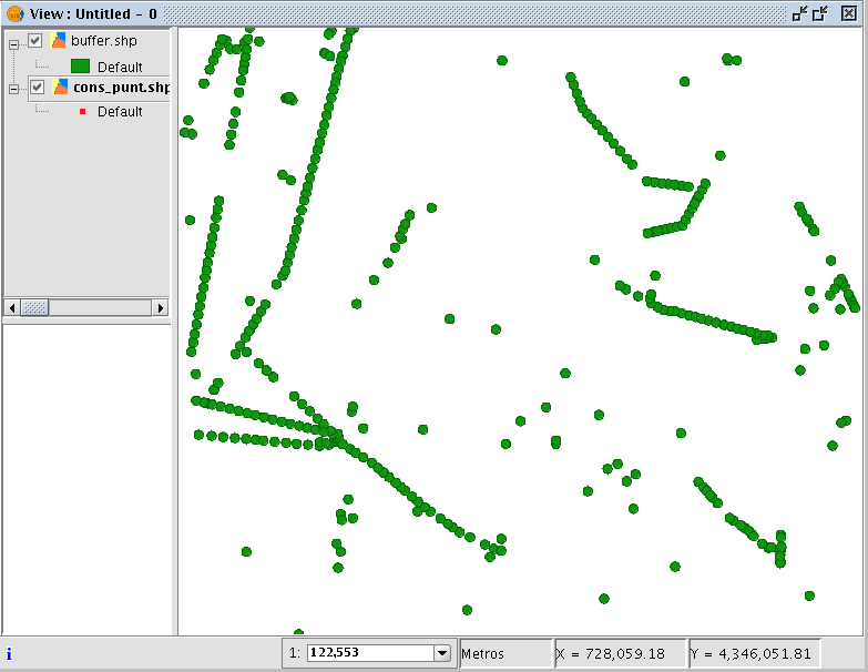
The process can be cancelled at any time by clicking on the “Cancel” button. As a consequence, the result file and any other intermediate product generated as a result of running the process are deleted. Whilst the buffer computing process is underway, other tasks can be carried out, such as changing the zoom or adding new layers to the layer tree in the gvSIG view. Other tasks can be carried out because all the geoprocessing extension geoprocesses are run in the background. When the process has finished, the new result layer is added to the layer tree in the active view. It is made up of buffer polygons with a specified radius based on the source layer.

Finally, the “Dissolve elements” option can be useful in specific situations (such as when the aim of computing the buffer polygons is to determine the total surface area affected by a phenomenon: quarantine areas, etc.), because when the generated polygons are merged the surface area covered by the buffer will be a real surface area, i.e. the sum of two buffers will not have any overlays.

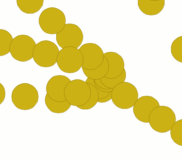
The above image shows non-merged overlay polygons. The total area covered by the phenomenon does not coincide with the sum of the individual areas.

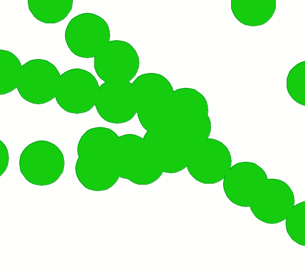
However, this second image shows merged overlay polygons. The total area covered by the phenomenon is real. When the buffer computing process includes the merger of overlay areas (dissolve) we cannot predict its exact duration (we do not know how many polygons will touch each other a priori). This is why the gvSIG geoprocessing extension does not show us a progress bar as such, it shows us a bar which periodically reaches the end and then goes back to the beginning. This type of process is called an “indeterminate” process.